Sharp regression discontinuity with scikit-learn models#

from sklearn.gaussian_process import GaussianProcessRegressor
from sklearn.gaussian_process.kernels import ExpSineSquared, WhiteKernel
from sklearn.linear_model import LinearRegression

import causalpy as cp

%config InlineBackend.figure_format = 'retina'

Load data#

data = cp.load_data("rd")
data.head(5)

	x	y	treated
0	-0.989008	-0.252433	False
1	-0.984119	-0.050974	False
2	-0.964955	-0.216572	False
3	-0.962408	-0.204497	False
4	-0.944821	-0.354276	False

Linear, main-effects model#

result = cp.RegressionDiscontinuity(
    data,
    formula="y ~ 1 + x + treated",
    model=LinearRegression(),
    treatment_threshold=0.5,
)

/Users/benjamv/git/CausalPy/causalpy/experiments/base.py:235: UserWarning: LinearRegression had fit_intercept=True, but CausalPy requires fit_intercept=False because the intercept is already included in the design matrix by patsy. A cloned copy of the model with fit_intercept=False will be used; the original instance is unchanged.

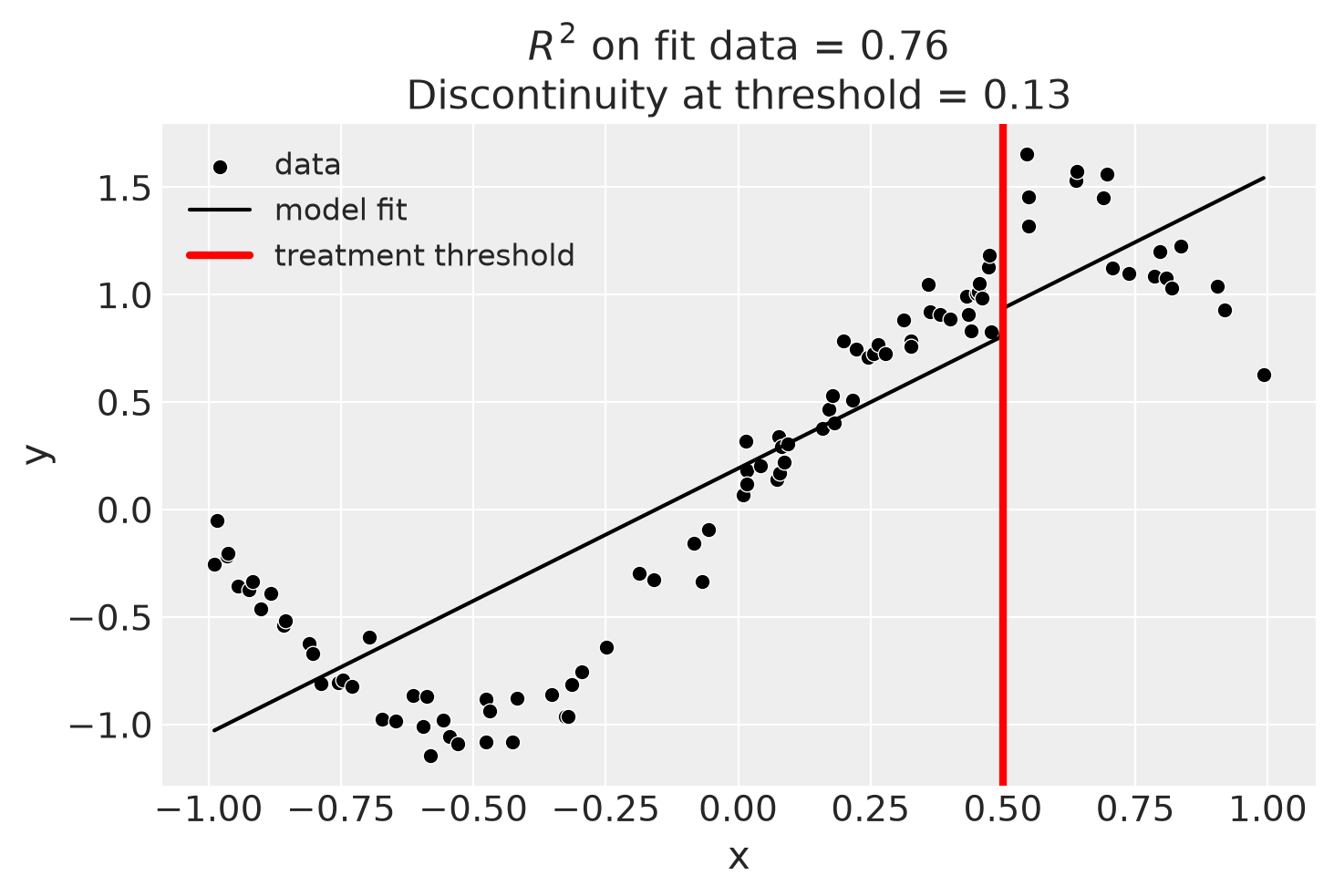
fig, ax = result.plot()

../_images/075d75a4308caaa190867e93ddb1a7f52400a57af4f5088b9dbf00a7f9ad06f2.png

result.summary(round_to=3)

Regression Discontinuity experiment
Formula: y ~ 1 + x + treated
Running variable: x
Threshold on running variable: 0.5
Bandwidth: inf
Donut hole: 0.0
Observations used for fit: 100

Results:
Discontinuity at threshold = 0.13


Model coefficients:
  Intercept      	     0.191
  treated[T.True]	     0.129
  x              	      1.23

We can get nicely formatted tables from our integration with the maketables package.

from maketables import ETable

ETable(result, coef_fmt="b:.3f")

	y
	(1)
coef
treated=True	0.129
x	1.233
Intercept	0.191
stats
N	100
R2	0.764
Format of coefficient cell: Coefficient

Linear, main-effects, and interaction model#

result = cp.RegressionDiscontinuity(
    data,
    formula="y ~ 1 + x + treated + x:treated",
    model=LinearRegression(),
    treatment_threshold=0.5,
)

/Users/benjamv/git/CausalPy/causalpy/experiments/base.py:235: UserWarning: LinearRegression had fit_intercept=True, but CausalPy requires fit_intercept=False because the intercept is already included in the design matrix by patsy. A cloned copy of the model with fit_intercept=False will be used; the original instance is unchanged.

result.plot();

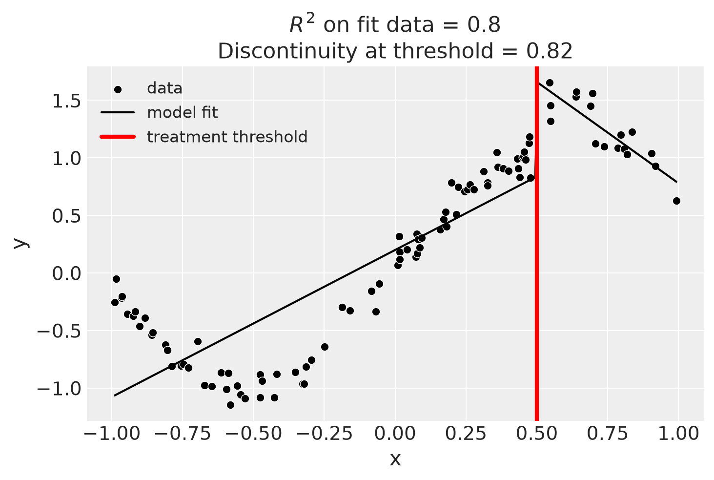
../_images/ffefea52d5bc73871594d8e581d131d0ad31207b7bc35db6105a41374cffde46.png

Though we can see that this does not give a good fit of the data almost certainly overestimates the discontinuity at threshold.

result.summary(round_to=3)

Regression Discontinuity experiment
Formula: y ~ 1 + x + treated + x:treated
Running variable: x
Threshold on running variable: 0.5
Bandwidth: inf
Donut hole: 0.0
Observations used for fit: 100

Results:
Discontinuity at threshold = 0.82


Model coefficients:
  Intercept        	       0.2
  treated[T.True]  	      2.34
  x                	      1.28
  x:treated[T.True]	     -3.04

Using a bandwidth#

One way how we could deal with this is to use the bandwidth kwarg. This will only fit the model to data within a certain bandwidth of the threshold. If \(x\) is the running variable, then the model will only be fitted to data where \(threshold - bandwidth \le x \le threshold + bandwidth\).

result = cp.RegressionDiscontinuity(
    data,
    formula="y ~ 1 + x + treated + x:treated",
    model=LinearRegression(),
    treatment_threshold=0.5,
    bandwidth=0.3,
)

result.plot();

/Users/benjamv/git/CausalPy/causalpy/experiments/base.py:235: UserWarning: LinearRegression had fit_intercept=True, but CausalPy requires fit_intercept=False because the intercept is already included in the design matrix by patsy. A cloned copy of the model with fit_intercept=False will be used; the original instance is unchanged.

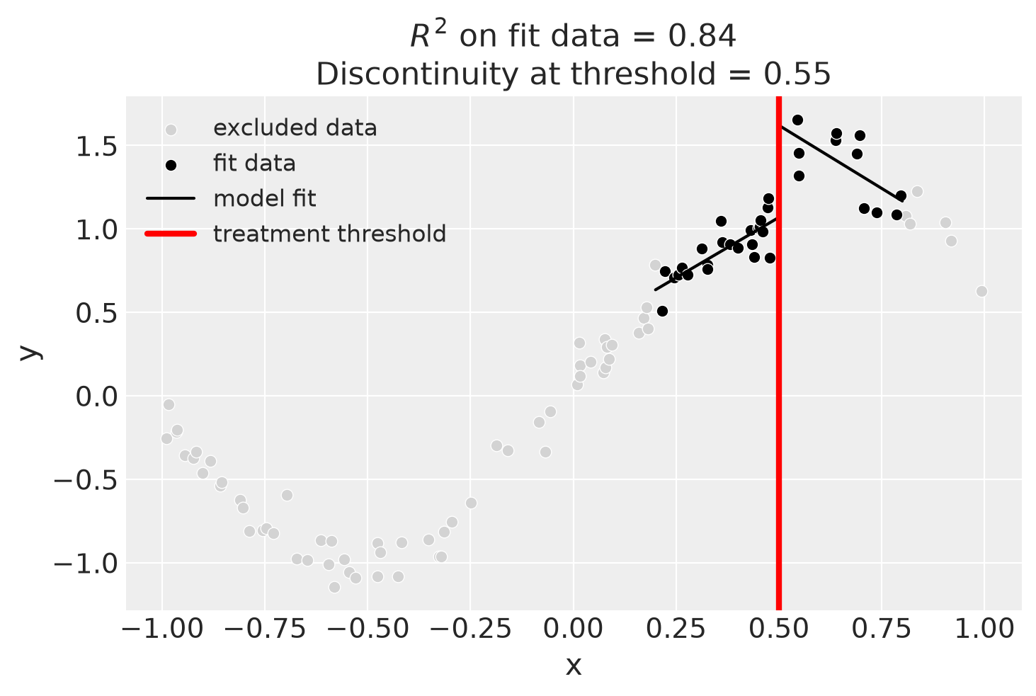
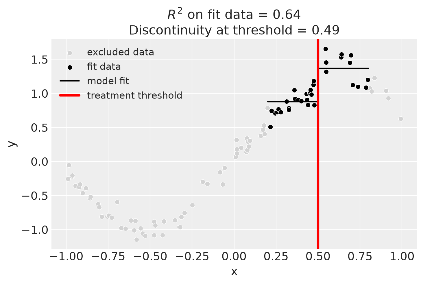
../_images/13113b84735e3ca8a85fcab2206e3ccf64a7559e5755834dc9bf4a6aab111270.png

We could even go crazy and just fit intercepts for the data close to the threshold. But clearly this will involve more estimation error as we are using less data.

result = cp.RegressionDiscontinuity(
    data,
    formula="y ~ 1 + treated",
    model=LinearRegression(),
    treatment_threshold=0.5,
    bandwidth=0.3,
)

result.plot();

/Users/benjamv/git/CausalPy/causalpy/experiments/base.py:235: UserWarning: LinearRegression had fit_intercept=True, but CausalPy requires fit_intercept=False because the intercept is already included in the design matrix by patsy. A cloned copy of the model with fit_intercept=False will be used; the original instance is unchanged.

../_images/aa8bded5dc27c9b7750aea1c3f4e397ee057874b065e515c3b4e9f0bcba4b6fb.png

Using Gaussian Processes#

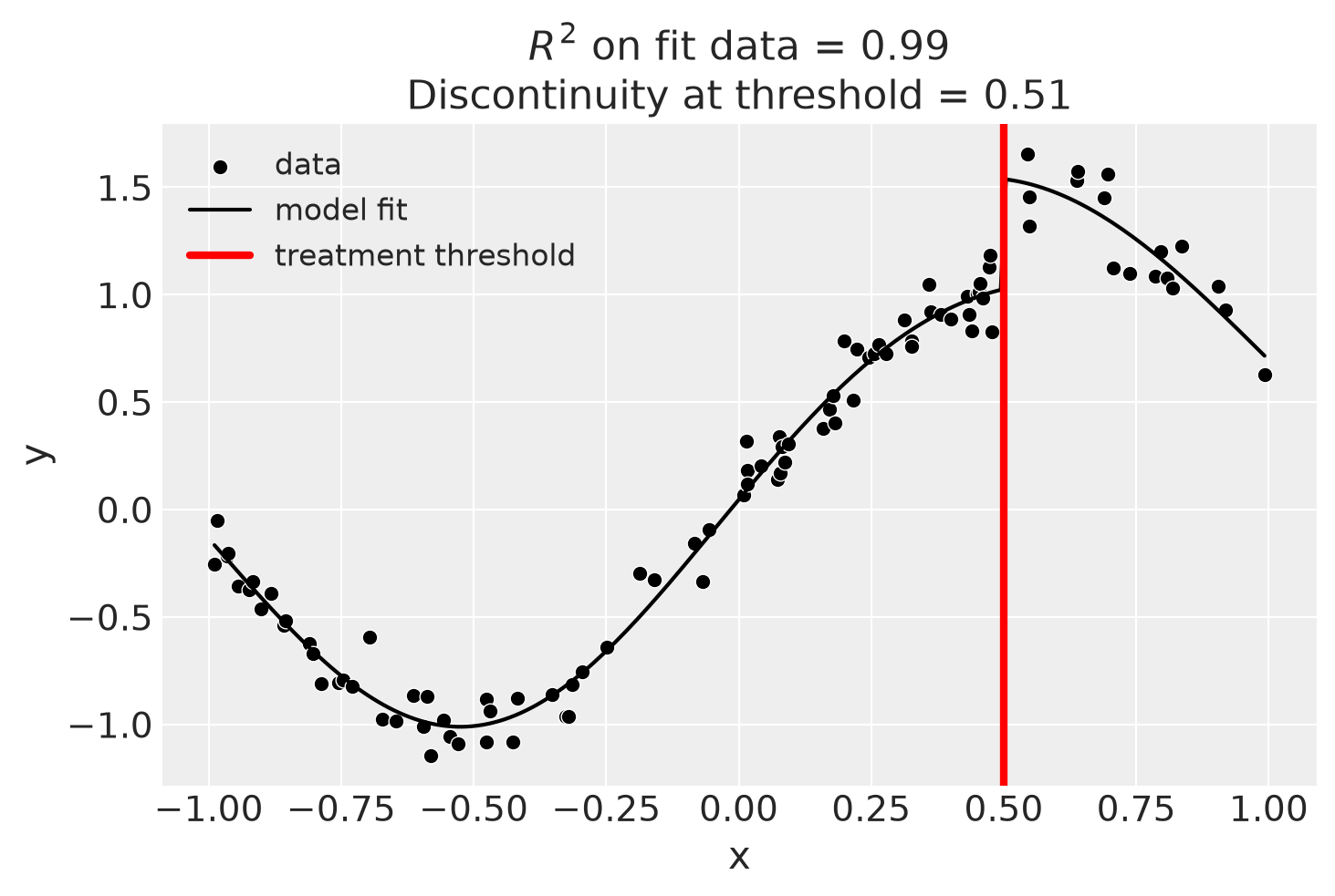
Now we will demonstrate how to use a scikit-learn model.

kernel = 1.0 * ExpSineSquared(1.0, 5.0) + WhiteKernel(1e-1)
result = cp.RegressionDiscontinuity(
    data,
    formula="y ~ 1 + x + treated",
    model=GaussianProcessRegressor(kernel=kernel),
    treatment_threshold=0.5,
)

fig, ax = result.plot()

../_images/56b77b2fc872c342a86b4d993a744e5ce098727d26e1fe6adfdf7277960ced27.png

Using basis splines#

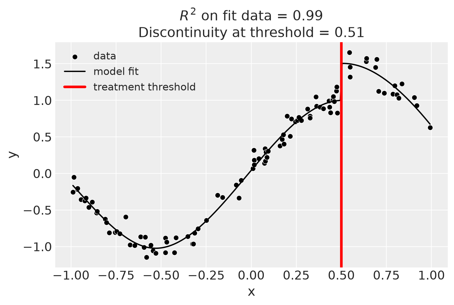
result = cp.RegressionDiscontinuity(
    data,
    formula="y ~ 1 + bs(x, df=6) + treated",
    model=LinearRegression(),
    treatment_threshold=0.5,
)

/Users/benjamv/git/CausalPy/causalpy/experiments/base.py:235: UserWarning: LinearRegression had fit_intercept=True, but CausalPy requires fit_intercept=False because the intercept is already included in the design matrix by patsy. A cloned copy of the model with fit_intercept=False will be used; the original instance is unchanged.

fig, ax = result.plot()

../_images/0e5793a212604b8aaa737764812fbb3111553c3819773bda320248af487776ba.png

result.summary(round_to=3)

Regression Discontinuity experiment
Formula: y ~ 1 + bs(x, df=6) + treated
Running variable: x
Threshold on running variable: 0.5
Bandwidth: inf
Donut hole: 0.0
Observations used for fit: 100

Results:
Discontinuity at threshold = 0.51


Model coefficients:
  Intercept      	    -0.165
  treated[T.True]	     0.505
  bs(x, df=6)[0] 	    -0.401
  bs(x, df=6)[1] 	     -1.42
  bs(x, df=6)[2] 	     0.268
  bs(x, df=6)[3] 	      1.51
  bs(x, df=6)[4] 	     0.892
  bs(x, df=6)[5] 	     0.334

Effect Summary Reporting#

For decision-making, you often need a concise summary of the causal effect. The effect_summary() method provides a decision-ready report with key statistics. Note that for Regression Discontinuity, the effect is a single scalar (the discontinuity at the threshold), similar to Difference-in-Differences.

Note

OLS vs PyMC Models: When using OLS models (scikit-learn), the effect_summary() provides confidence intervals and p-values (frequentist inference), rather than the posterior distributions, HDI intervals, and tail probabilities provided by PyMC models (Bayesian inference). OLS tables include: mean, CI_lower, CI_upper, and p_value, but do not include median, tail probabilities (P(effect>0)), or ROPE probabilities.

# Generate effect summary for the final model (basis splines)
stats = result.effect_summary()
stats.table

	mean	ci_lower	ci_upper	p_value
discontinuity	0.505527	0.273907	0.737147	0.000037

# View the prose summary
print(stats.text)

The discontinuity at threshold was 0.51 (95% CI [0.27, 0.74]), with a p-value of 0.000.

# You can specify the direction of interest (e.g., testing for an increase)
stats_increase = result.effect_summary(direction="increase")
stats_increase.table

	mean	ci_lower	ci_upper	p_value
discontinuity	0.505527	0.273907	0.737147	0.000037