Difference in Differences with scikit-learn models

from sklearn.linear_model import LinearRegression

import causalpy as cp

data = cp.load_data("did")

result = cp.DifferenceInDifferences(
    data,
    formula="y ~ 1 + group*post_treatment",
    time_variable_name="t",
    group_variable_name="group",
    model=LinearRegression(),
)

/Users/benjamv/git/CausalPy/causalpy/experiments/base.py:235: UserWarning: LinearRegression had fit_intercept=True, but CausalPy requires fit_intercept=False because the intercept is already included in the design matrix by patsy. A cloned copy of the model with fit_intercept=False will be used; the original instance is unchanged.

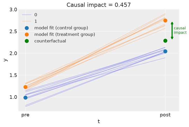
fig, ax = result.plot(round_to=3)

result.summary(round_to=3)

===========================Difference in Differences============================
Formula: y ~ 1 + group*post_treatment

Results:
Causal impact = 0.46
Model coefficients:
  Intercept                   	     0.988
  post_treatment[T.True]      	      1.06
  group                       	     0.242
  group:post_treatment[T.True]	     0.457

We can get nicely formatted tables from our integration with the maketables package.

from maketables import ETable

ETable(result, coef_fmt="b:.3f")

	y
	(1)
coef
post_treatment=True	1.058
group	0.242
group × post_treatment=True	0.457
Intercept	0.988
stats
N	40
Format of coefficient cell: Coefficient

Effect Summary Reporting

For decision-making, you often need a concise summary of the causal effect. The effect_summary() method provides a decision-ready report with key statistics. Note that for Difference-in-Differences, the effect is a single scalar (average treatment effect), unlike time-series experiments where effects vary over time.

Note

OLS vs PyMC Models: When using OLS models (scikit-learn), the effect_summary() provides confidence intervals and p-values (frequentist inference), rather than the posterior distributions, HDI intervals, and tail probabilities provided by PyMC models (Bayesian inference). OLS tables include: mean, CI_lower, CI_upper, and p_value, but do not include median, tail probabilities (P(effect>0)), or ROPE probabilities.

# Generate effect summary
stats = result.effect_summary()
stats.table

	mean	ci_lower	ci_upper	p_value
treatment_effect	0.457139	-0.80812	1.722398	0.468454

# View the prose summary
print(stats.text)

The treatment effect was 0.46 (95% CI [-0.81, 1.72]), with a p-value of 0.468.

# You can specify the direction of interest (e.g., testing for an increase)
stats_increase = result.effect_summary(direction="increase")
stats_increase.table

	mean	ci_lower	ci_upper	p_value
treatment_effect	0.457139	-0.80812	1.722398	0.468454