Interrupted Time Series (ITS) with scikit-learn models

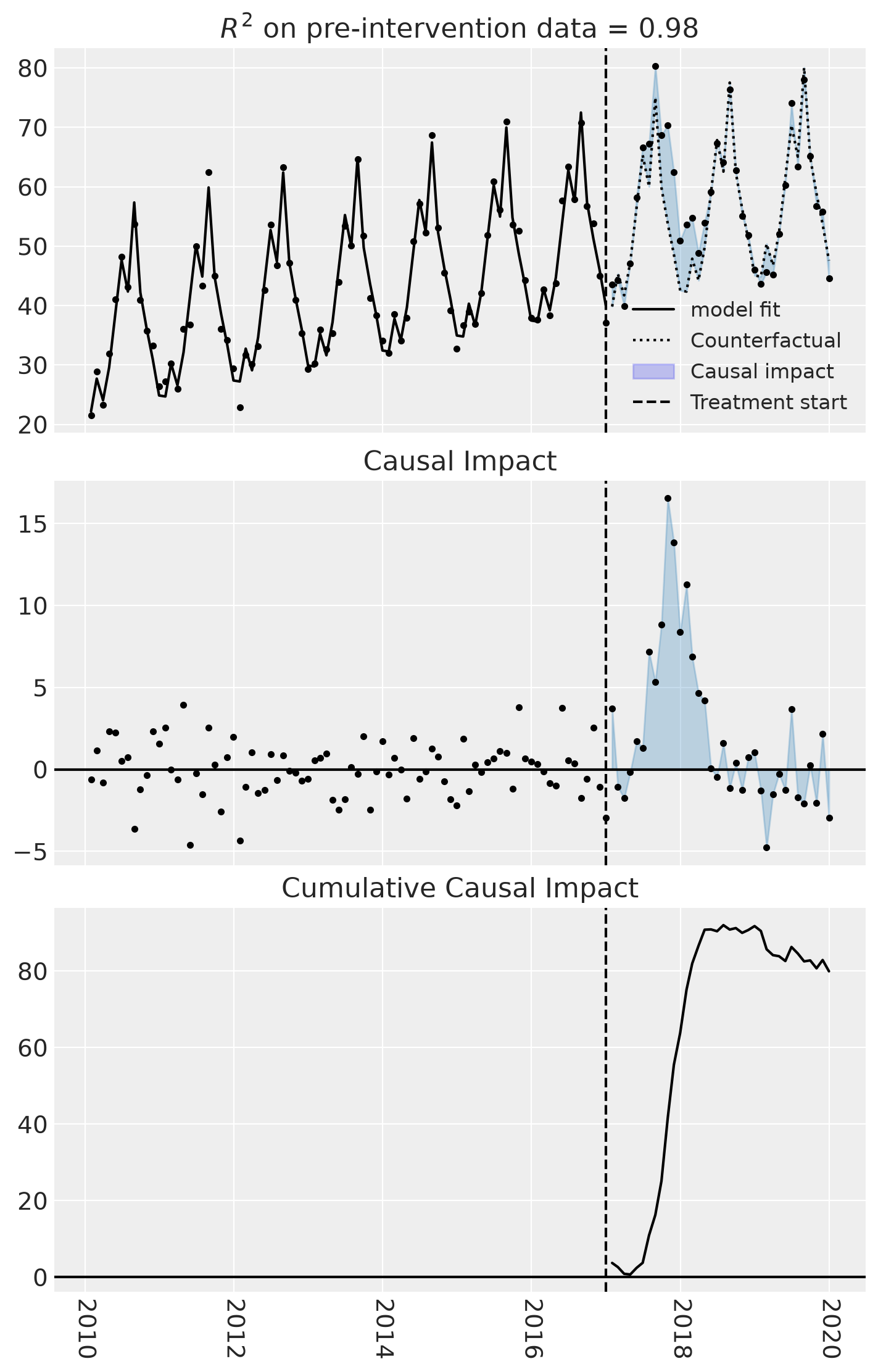
This notebook shows an example of using interrupted time series, where we do not have untreated control units of a similar nature to the treated unit and we just have a single time series of observations and the predictor variables are simply time and month.

import pandas as pd
from sklearn.linear_model import LinearRegression

import causalpy as cp

%config InlineBackend.figure_format = 'retina'

Load data

df = (
    cp.load_data("its")
    .assign(date=lambda x: pd.to_datetime(x["date"]))
    .set_index("date")
)

treatment_time = pd.to_datetime("2017-01-01")
df.head(5)

	year	month	t	y	causal effect	intercept
date
2010-01-31	2010	1	0	21.554716	0.0	1.0
2010-02-28	2010	2	1	28.851317	0.0	1.0
2010-03-31	2010	3	2	23.258060	0.0	1.0
2010-04-30	2010	4	3	31.936498	0.0	1.0
2010-05-31	2010	5	4	41.090762	0.0	1.0

Run the analysis

result = cp.InterruptedTimeSeries(
    df,
    treatment_time,
    formula="y ~ 1 + t + C(month)",
    model=LinearRegression(),
)

/Users/benjamv/git/CausalPy/causalpy/experiments/base.py:235: UserWarning: LinearRegression had fit_intercept=True, but CausalPy requires fit_intercept=False because the intercept is already included in the design matrix by patsy. A cloned copy of the model with fit_intercept=False will be used; the original instance is unchanged.

Examine the results

fig, ax = result.plot()

result.summary(round_to=3)

==================================Pre-Post Fit==================================
Formula: y ~ 1 + t + C(month)
Model coefficients:
  Intercept     	      22.2
  C(month)[T.2] 	      5.31
  C(month)[T.3] 	      1.46
  C(month)[T.4] 	       6.8
  C(month)[T.5] 	      15.8
  C(month)[T.6] 	      24.4
  C(month)[T.7] 	      18.9
  C(month)[T.8] 	      33.7
  C(month)[T.9] 	      18.3
  C(month)[T.10]	      12.1
  C(month)[T.11]	      6.67
  C(month)[T.12]	     0.374
  t             	      0.21

We can get nicely formatted tables from our integration with the maketables package.

from maketables import ETable

ETable(result, coef_fmt="b:.3f")

	y
	(1)
coef
month=2	5.314
month=3	1.457
month=4	6.803
month=5	15.811
month=6	24.438
month=7	18.920
month=8	33.702
month=9	18.341
month=10	12.053
month=11	6.670
month=12	0.374
t	0.210
Intercept	22.179
stats
N	120
R2	0.979
Format of coefficient cell: Coefficient

Effect Summary Reporting

For decision-making, you often need a concise summary of the causal effect. The effect_summary() method provides a decision-ready report with key statistics.

Note

OLS vs PyMC Models: When using OLS models (scikit-learn), the effect_summary() provides confidence intervals and p-values (frequentist inference), rather than the posterior distributions, HDI intervals, and tail probabilities provided by PyMC models (Bayesian inference). OLS tables include: mean, CI_lower, CI_upper, and p_value, but do not include median, tail probabilities (P(effect>0)), or ROPE probabilities.

# Generate effect summary for the full post-period
stats = result.effect_summary()
stats.table

	mean	ci_lower	ci_upper	p_value	relative_mean	relative_ci_lower	relative_ci_upper
average	2.220331	0.576604	3.864058	0.009551	4.420944	1.129960	7.711929
cumulative	79.931912	20.757728	139.106096	0.009551	159.153997	40.678565	277.629429

# View the prose summary
print(stats.text)

During the Post-period (2017-01-31 00:00:00 to 2019-12-31 00:00:00), the response variable had an average value of approx. 57.73. By contrast, in the absence of an intervention, we would have expected an average response of 55.51. The 95% confidence interval of this counterfactual prediction is [53.87, 57.16]. Subtracting this prediction from the observed response yields an estimate of the causal effect the intervention had on the response variable. This effect is 2.22 with a 95% confidence interval of [0.58, 3.86].

Summing up the individual data points during the Post-period, the response variable had an overall value of 2078.37. By contrast, had the intervention not taken place, we would have expected a sum of 1998.44. The 95% confidence interval of this prediction is [1939.26, 2057.61].

The 95% confidence interval of the effect [0.58, 3.86] does not include zero (p-value 0.010). Relative to the counterfactual, the effect represents a 4.42% change (95% CI [1.13%, 7.71%]).

This analysis assumes that the relationship between the time-based predictors and the response observed during the pre-intervention period remains stable throughout the post-intervention period. If the formula includes external covariates, it further assumes they were not themselves affected by the intervention. We recommend inspecting model fit, examining pre-intervention trends, and conducting sensitivity analyses (e.g., placebo tests) to support any causal conclusions drawn from this analysis.