Sharp regression discontinuity with `pymc` models#

import causalpy as cp

%load_ext autoreload
%autoreload 2
%config InlineBackend.figure_format = 'retina'
seed = 42

df = cp.load_data("rd")

Linear, main-effects, and interaction model#

Note

The random_seed keyword argument for the PyMC sampler is not necessary. We use it here so that the results are reproducible.

result = cp.RegressionDiscontinuity(
    df,
    formula="y ~ 1 + x + treated + x:treated",
    model=cp.pymc_models.LinearRegression(sample_kwargs={"random_seed": seed}),
    treatment_threshold=0.5,
)

fig, ax = result.plot(show=False)
fig

Initializing NUTS using jitter+adapt_diag...

Multiprocess sampling (4 chains in 4 jobs)

NUTS: [beta, y_hat_sigma]

Sampling 4 chains for 1_000 tune and 1_000 draw iterations (4_000 + 4_000 draws total) took 1 seconds.

Sampling: [beta, y_hat, y_hat_sigma]

Sampling: [y_hat]

Sampling: [y_hat]

Sampling: [y_hat]

Sampling: [y_hat]

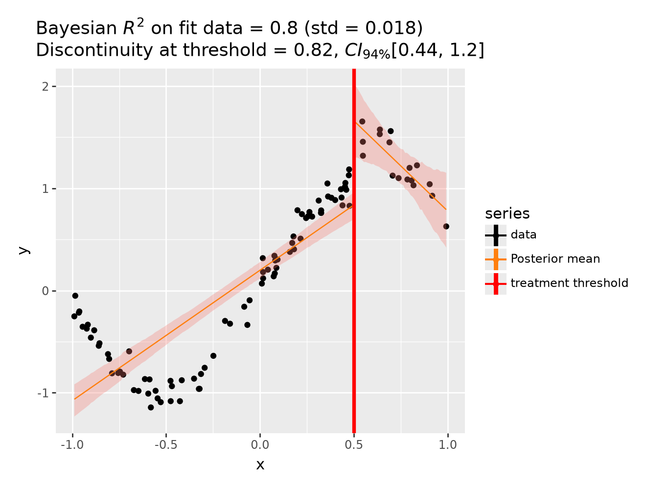
../_images/43cba9af111b54b8669f2a95ab0d1bc26203fd6adddc730688a425dad00c94d6.png

Though we can see that this does not give a good fit of the data almost certainly overestimates the discontinuity at threshold.

Using a bandwidth#

One way how we could deal with this is to use the bandwidth kwarg. This will only fit the model to data within a certain bandwidth of the threshold. If \(x\) is the running variable, then the model will only be fitted to data where \(threshold - bandwidth \le x \le threshold + bandwidth\).

result = cp.RegressionDiscontinuity(
    df,
    formula="y ~ 1 + x + treated + x:treated",
    model=cp.pymc_models.LinearRegression(sample_kwargs={"random_seed": seed}),
    treatment_threshold=0.5,
    bandwidth=0.3,
)

result.plot()

Initializing NUTS using jitter+adapt_diag...

Multiprocess sampling (4 chains in 4 jobs)

NUTS: [beta, y_hat_sigma]

Sampling 4 chains for 1_000 tune and 1_000 draw iterations (4_000 + 4_000 draws total) took 2 seconds.

Sampling: [beta, y_hat, y_hat_sigma]

Sampling: [y_hat]

Sampling: [y_hat]

Sampling: [y_hat]

Sampling: [y_hat]

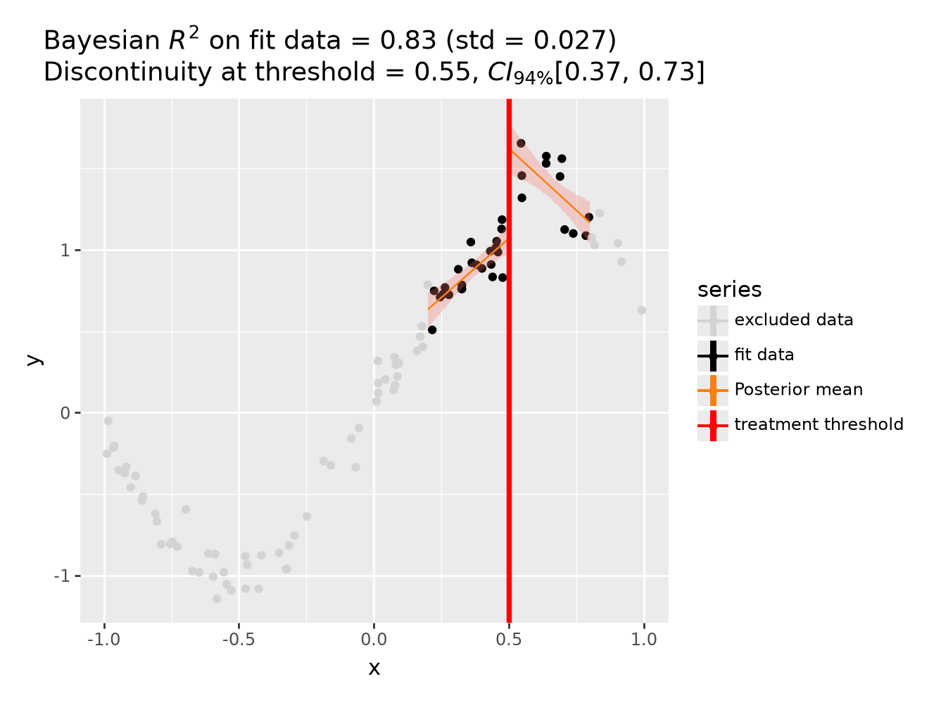
../_images/0f64674fb326d9c5653405f31b74805dc8aec63ca133f3be7635d34e1dc404dc.png

(<Figure size 640x480 with 1 Axes>, <Axes: >)

We could even go crazy and just fit intercepts for the data close to the threshold. But clearly this will involve more estimation error as we are using less data.

result = cp.RegressionDiscontinuity(
    df,
    formula="y ~ 1 + treated",
    model=cp.pymc_models.LinearRegression(sample_kwargs={"random_seed": seed}),
    treatment_threshold=0.5,
    bandwidth=0.2,
)

result.plot()

Initializing NUTS using jitter+adapt_diag...

Multiprocess sampling (4 chains in 4 jobs)

NUTS: [beta, y_hat_sigma]

Sampling 4 chains for 1_000 tune and 1_000 draw iterations (4_000 + 4_000 draws total) took 0 seconds.

Sampling: [beta, y_hat, y_hat_sigma]

Sampling: [y_hat]

Sampling: [y_hat]

Sampling: [y_hat]

Sampling: [y_hat]

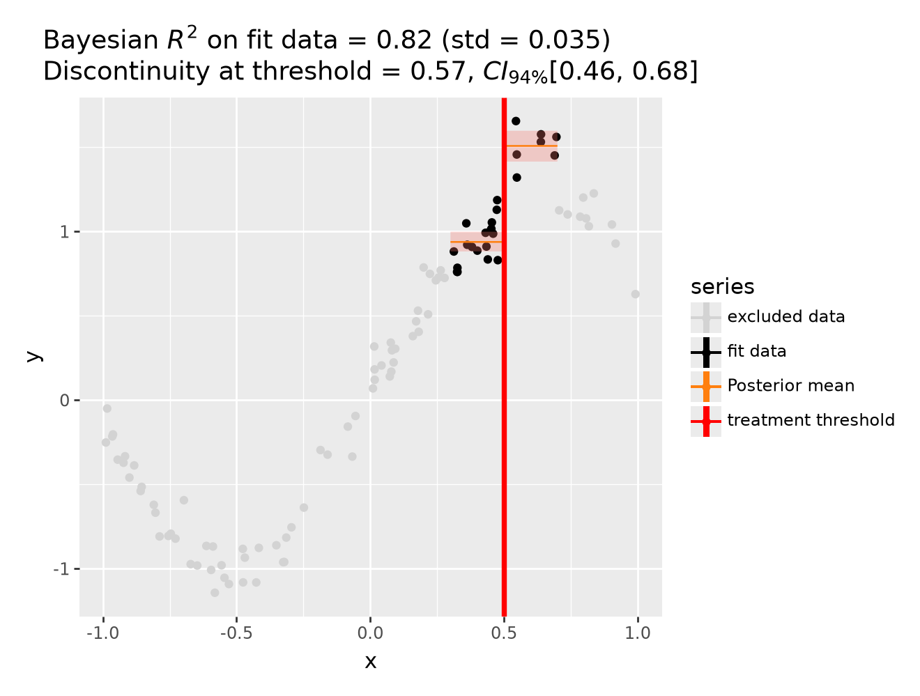
../_images/83e1aa7abe3b6d7b72013f2b9e3d3be65b636dfb31fc69dba35f6b7e06f0478e.png

(<Figure size 640x480 with 1 Axes>, <Axes: >)

Using basis splines#

Though it could arguably be better to fit with a more complex model, fit example a spline. This allows us to use all of the data, and (depending on the situation) maybe give a better fit.

result = cp.RegressionDiscontinuity(
    df,
    formula="y ~ 1 + bs(x, df=6) + treated",
    model=cp.pymc_models.LinearRegression(sample_kwargs={"random_seed": seed}),
    treatment_threshold=0.5,
)

result.plot()

Initializing NUTS using jitter+adapt_diag...

Multiprocess sampling (4 chains in 4 jobs)

NUTS: [beta, y_hat_sigma]

Sampling 4 chains for 1_000 tune and 1_000 draw iterations (4_000 + 4_000 draws total) took 1 seconds.

Sampling: [beta, y_hat, y_hat_sigma]

Sampling: [y_hat]

Sampling: [y_hat]

Sampling: [y_hat]

Sampling: [y_hat]

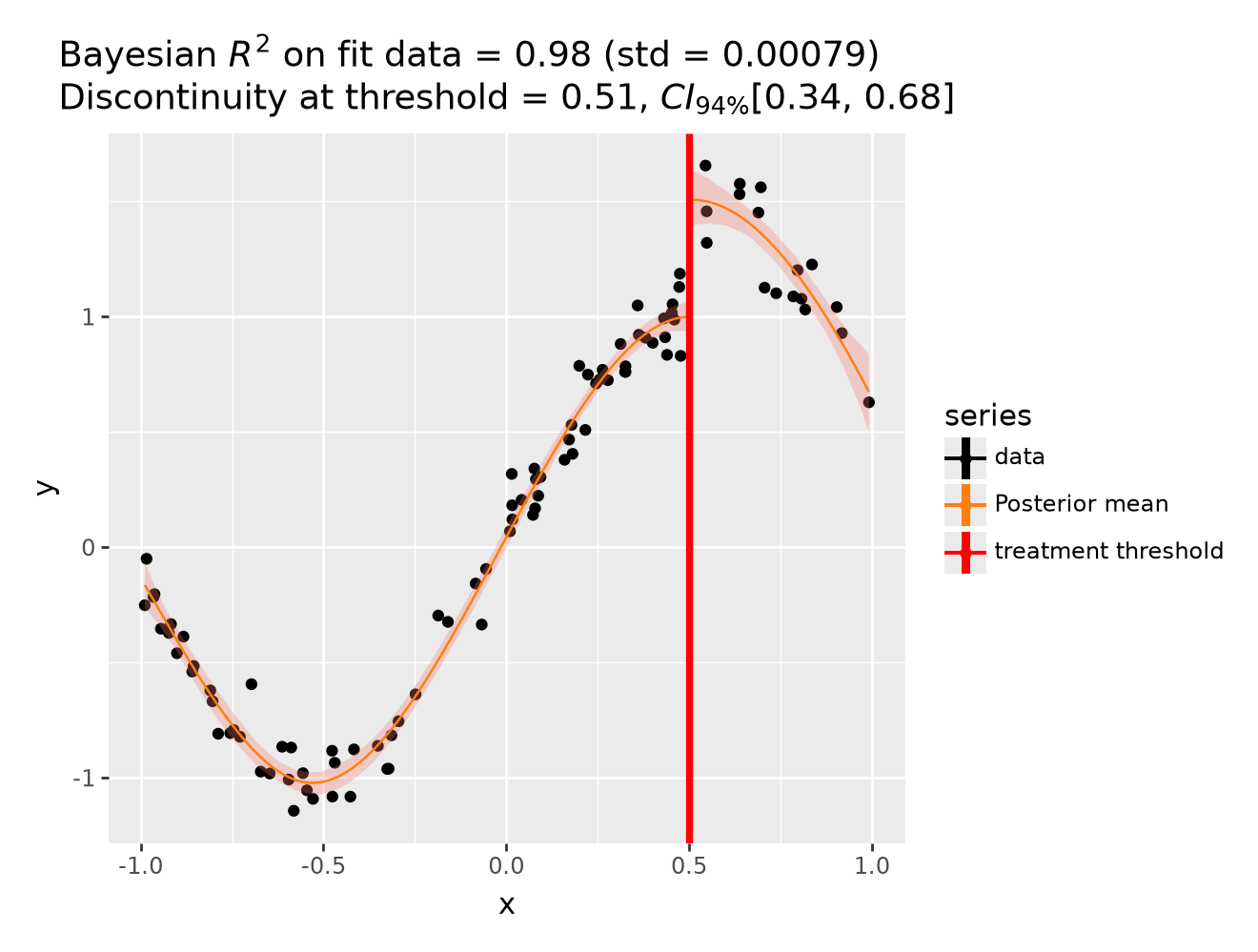
../_images/74dd782e5c29208aeaf1de1c85c5821a6ec5bd54aecf6ea7c61406b0491b0beb.png

(<Figure size 640x480 with 1 Axes>, <Axes: >)

As with all of the models in this notebook, we can ask for a summary of the model coefficients.

result.summary()

Regression Discontinuity experiment
Formula: y ~ 1 + bs(x, df=6) + treated
Running variable: x
Threshold on running variable: 0.5
Bandwidth: inf
Donut hole: 0.0
Observations used for fit: 100

Results:
Discontinuity at threshold = 0.51$CI_{94\%}$[0.34, 0.68]


Model coefficients:
    Intercept        -0.16, 94% HDI [-0.26, -0.065]
    treated[T.True]  0.51, 94% HDI [0.34, 0.68]
    bs(x, df=6)[0]   -0.4, 94% HDI [-0.6, -0.2]
    bs(x, df=6)[1]   -1.4, 94% HDI [-1.6, -1.3]
    bs(x, df=6)[2]   0.27, 94% HDI [0.11, 0.43]
    bs(x, df=6)[3]   1.5, 94% HDI [1.4, 1.7]
    bs(x, df=6)[4]   0.89, 94% HDI [0.53, 1.3]
    bs(x, df=6)[5]   0.33, 94% HDI [0.1, 0.55]
    y_hat_sigma      0.11, 94% HDI [0.093, 0.12]

We can get nicely formatted tables from our integration with the maketables package.

from maketables import ETable

result.set_maketables_options(hdi_prob=0.95)
ETable(result, coef_fmt="b:.3f \n [ci95l:.3f, ci95u:.3f]")

	y
	(1)
coef
treated=True	0.506 [0.331, 0.680]
bs(x, df=6)=0	-0.403 [-0.604, -0.187]
bs(x, df=6)=1	-1.425 [-1.577, -1.272]
bs(x, df=6)=2	0.267 [0.101, 0.436]
bs(x, df=6)=3	1.507 [1.347, 1.660]
bs(x, df=6)=4	0.890 [0.520, 1.280]
bs(x, df=6)=5	0.331 [0.073, 0.541]
Intercept	-0.164 [-0.266, -0.058]
stats
N	100
Bayesian R2	0.984
Format of coefficient cell: Coefficient [95% CI Lower, 95% CI Upper]

Effect Summary Reporting#

For decision-making, you often need a concise summary of the causal effect. The effect_summary() method provides a decision-ready report with key statistics. Note that for Regression Discontinuity, the effect is a single scalar (the discontinuity at the threshold), similar to Difference-in-Differences.

# Generate effect summary
stats = result.effect_summary()
stats.table

	mean	median	hdi_lower	hdi_upper	p_gt_0
discontinuity	0.506269	0.50609	0.332965	0.679456	1.0

print(stats.text)

The discontinuity at threshold was 0.51 (95% HDI [0.33, 0.68]), with a posterior probability of an increase of 1.000.

You can customize the summary with different directions and ROPE thresholds:

Direction: Test for increase, decrease, or two-sided effect
Alpha: Set the HDI confidence level (default 95%)
ROPE: Specify a minimal effect size threshold

# Example: Two-sided test with ROPE
stats = result.effect_summary(
    direction="two-sided",
    alpha=0.05,
    min_effect=0.2,  # Region of Practical Equivalence
)
stats.table

	mean	median	hdi_lower	hdi_upper	p_two_sided	prob_of_effect	p_rope
discontinuity	0.506269	0.50609	0.332965	0.679456	0.0	1.0	1.0

print("\n" + stats.text)

The discontinuity at threshold was 0.51 (95% HDI [0.33, 0.68]), with a posterior probability of an effect of 1.000.

Sharp regression discontinuity with pymc models#