Difference in Differences with `pymc` models#

Note

This example is in-progress! Further elaboration and explanation will follow soon.

import arviz as az

import causalpy as cp

%load_ext autoreload
%autoreload 2
%config InlineBackend.figure_format = 'retina'
seed = 42

Load data#

df = cp.load_data("did")
df.head()

	group	t	unit	post_treatment	y
0	0	0.0	0	False	0.977736
1	0	1.0	0	True	2.132566
2	1	0.0	1	False	1.192903
3	1	1.0	1	True	2.816825
4	0	0.0	2	False	1.114538

Run the analysis#

Note

The random_seed keyword argument for the PyMC sampler is not necessary. We use it here so that the results are reproducible.

result = cp.DifferenceInDifferences(
    df,
    formula="y ~ 1 + group*post_treatment",
    time_variable_name="t",
    group_variable_name="group",
    model=cp.pymc_models.LinearRegression(sample_kwargs={"random_seed": seed}),
)

Initializing NUTS using jitter+adapt_diag...

Multiprocess sampling (4 chains in 4 jobs)

NUTS: [beta, y_hat_sigma]

Sampling 4 chains for 1_000 tune and 1_000 draw iterations (4_000 + 4_000 draws total) took 1 seconds.

Sampling: [beta, y_hat, y_hat_sigma]

Sampling: [y_hat]

Sampling: [y_hat]

Sampling: [y_hat]

Sampling: [y_hat]

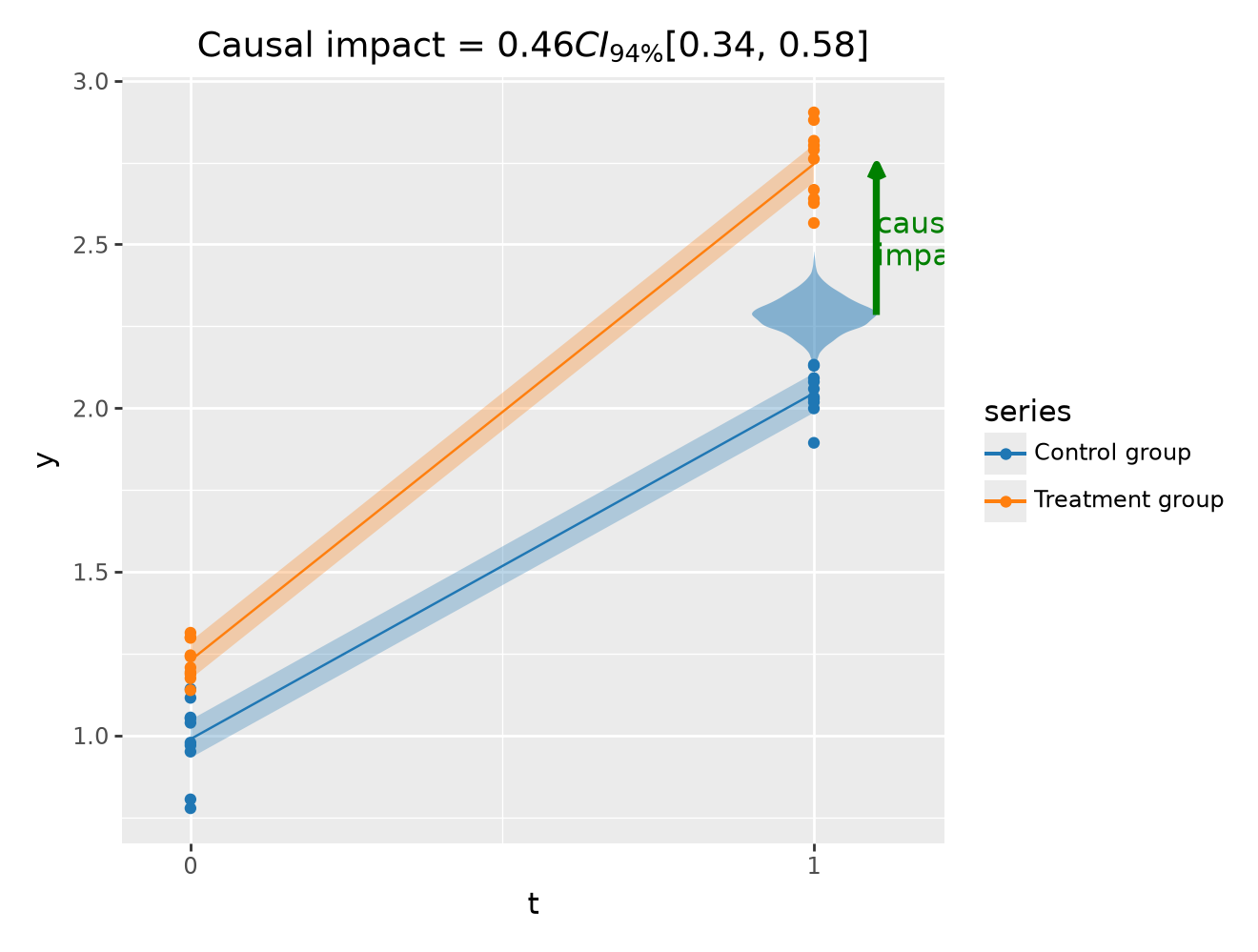
fig, ax = result.plot()

../_images/ef38ab491a056c5053e0c39f9bcd6efcfa408fa57a8dd53254c033e51ad876f7.png

result.summary()

===========================Difference in Differences============================
Formula: y ~ 1 + group*post_treatment

Results:
Causal impact = 0.46$CI_{94\%}$[0.34, 0.58]
Model coefficients:
    Intercept                     0.99, 94% HDI [0.93, 1]
    post_treatment[T.True]        1.1, 94% HDI [0.97, 1.1]
    group                         0.24, 94% HDI [0.16, 0.32]
    group:post_treatment[T.True]  0.46, 94% HDI [0.34, 0.58]
    y_hat_sigma                   0.098, 94% HDI [0.079, 0.12]

We can get nicely formatted tables from our integration with the maketables package.

from maketables import ETable

result.set_maketables_options(hdi_prob=0.95)
ETable(result, coef_fmt="b:.3f \n [ci95l:.3f, ci95u:.3f]")

	y
	(1)
coef
post_treatment=True	1.057 [0.971, 1.144]
group	0.240 [0.154, 0.324]
group × post_treatment=True	0.460 [0.343, 0.586]
Intercept	0.988 [0.927, 1.048]
stats
N	40
Format of coefficient cell: Coefficient [95% CI Lower, 95% CI Upper]

ax = az.plot_posterior(result.causal_impact, ref_val=0)
ax.set(title="Posterior estimate of causal impact");

Effect Summary Reporting#

For decision-making, you often need a concise summary of the causal effect. The effect_summary() method provides a decision-ready report with key statistics. Note that for Difference-in-Differences, the effect is a single scalar (average treatment effect), unlike time-series experiments where effects vary over time.

# Generate effect summary
stats = result.effect_summary()
stats.table

	mean	median	hdi_lower	hdi_upper	p_gt_0
treatment_effect	0.459532	0.458408	0.34271	0.585747	1.0

print(stats.text)

The average treatment effect was 0.46 (95% HDI [0.34, 0.59]), with a posterior probability of an increase of 1.000.

You can customize the summary with different directions and ROPE thresholds:

Direction: Test for increase, decrease, or two-sided effect
Alpha: Set the HDI confidence level (default 95%)
ROPE: Specify a minimal effect size threshold

# Example: Two-sided test with ROPE
stats = result.effect_summary(
    direction="two-sided",
    alpha=0.05,
    min_effect=0.3,  # Region of Practical Equivalence
)
stats.table

	mean	median	hdi_lower	hdi_upper	p_two_sided	prob_of_effect	p_rope
treatment_effect	0.459532	0.458408	0.34271	0.585747	0.0	1.0	0.995

print("\n" + stats.text)

The average treatment effect was 0.46 (95% HDI [0.34, 0.59]), with a posterior probability of an effect of 1.000.

Difference in Differences with pymc models#

Load data#

Run the analysis#

Effect Summary Reporting#

Difference in Differences with `pymc` models#